Import
Import is where a project becomes usable. Add the source files, let Niamoto detect their roles, review the generated configuration, then load the data into the project workspace.
What this stage controls
Use Import to:
add CSV tables, spatial layers, and rasters
review detected identifiers and source roles
edit the generated configuration before import
run the import and confirm the project is ready for Collections
If you are still at the very beginning, pair this page with ../01-getting-started/first-project.md.
1. Add the source files
Start from the dashboard or the Import area and select the files that belong to the project.
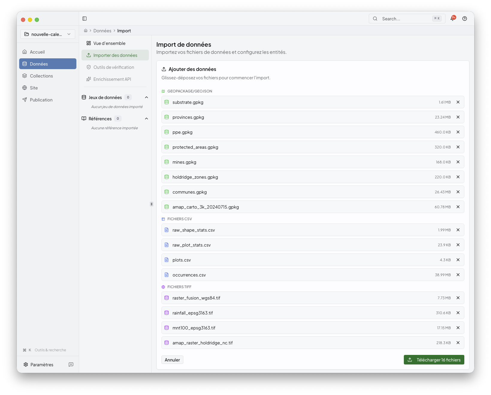
The desktop app now keeps a single import cockpit visible while you work. The same file inventory follows the batch from selection to analysis, review, and import, so you do not need to compare several separate lists.
Typical inputs include:
CSV tables
GeoPackage or GeoJSON layers
TIFF rasters
If your source is a shapefile, prefer converting it to GeoPackage when possible. The desktop upload accepts zipped shapefile packages, but the automatic import configuration is most reliable with GeoPackage or GeoJSON spatial layers.
The import screen uses a preparation assistant with a section selector on the left and contextual guidance on the right. Start with the overview, open Files and models when you want starter CSV templates, use Key checks to verify the minimum structure, and keep Advanced details for nested hierarchies or precomputed class/value data.
When you select files, Niamoto also runs a lightweight local preview before upload. This does not import anything yet; it checks whether CSV headers are readable, whether likely identifier columns exist, and whether the file looks like a hierarchy or a class/value table. These hints appear as one status per file in the cockpit; open a file in the side panel when you want the detailed checks.
For the most reliable automatic detection:
keep one clear header row in CSV files
use explicit identifier columns such as
id,plot_id, ortaxon_idreuse the same identifier values between related files
prefer GeoPackage or GeoJSON for spatial data
The same help area provides starter CSV templates next to the relevant choice:
one for occurrences with embedded taxonomy and one for site or plot references.
The class_object template is kept inside the advanced class/value panel so it
does not distract from the standard import path.
If your data have nested levels, open the hierarchy help panel before upload.
In the standard taxonomy workflow, you usually do not need a separate taxonomy
file: Niamoto can derive the taxonomic reference from the occurrences CSV when
it includes columns such as id_taxonref, taxaname, family, genus,
species, and infra. Niamoto detects taxonomic and geographic hierarchies
best when each level has its own column, with at least two levels in the same
CSV. Use clear names such as family, genus, species, country, region,
locality, or plot, and keep the levels ordered from broad to precise.
Stable identifiers such as taxon_id, plot_id, id_taxon, or id help
Niamoto link the hierarchy back to other files.
If you have values already calculated by class, open the class_object help
panel before upload. This format is for rows that attach one entity to one
measured object, an optional class, and one numeric value. For example, one row
can mean: plot plot_001 has 8.4 units of forest_cover in the forest
class.
That file must include the columns class_object, class_name, and
class_value; it also needs an entity identifier column named entity_id,
plot_id, shape_id, taxon_id, or id. Values in class_value must be
numeric. The desktop app provides a downloadable CSV template from the same help
panel.
2. Let Niamoto analyse the files
After selection, Niamoto runs live analysis and updates the same cockpit in place.
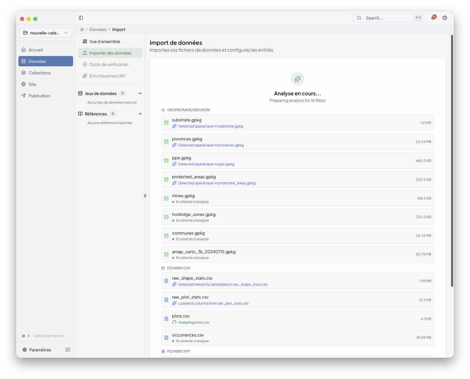
This stage is where the app tries to recognise:
main datasets
reference entities
supporting sources
layers or auxiliary files that should stay attached to a collection
Large batches are grouped by role when possible: occurrences, Sites/Parcelles, class/value tables, spatial layers, rasters, reference tables, and supporting tables. Repeated files such as many GeoPackage layers are grouped so the main screen stays scannable.
You do not need to understand the ML pipeline to use this step, but if you want the deeper explanation, see ../05-ml-detection/README.md.
3. Review the generated configuration
When analysis finishes, the cockpit shows what Niamoto inferred and what still needs confirmation.
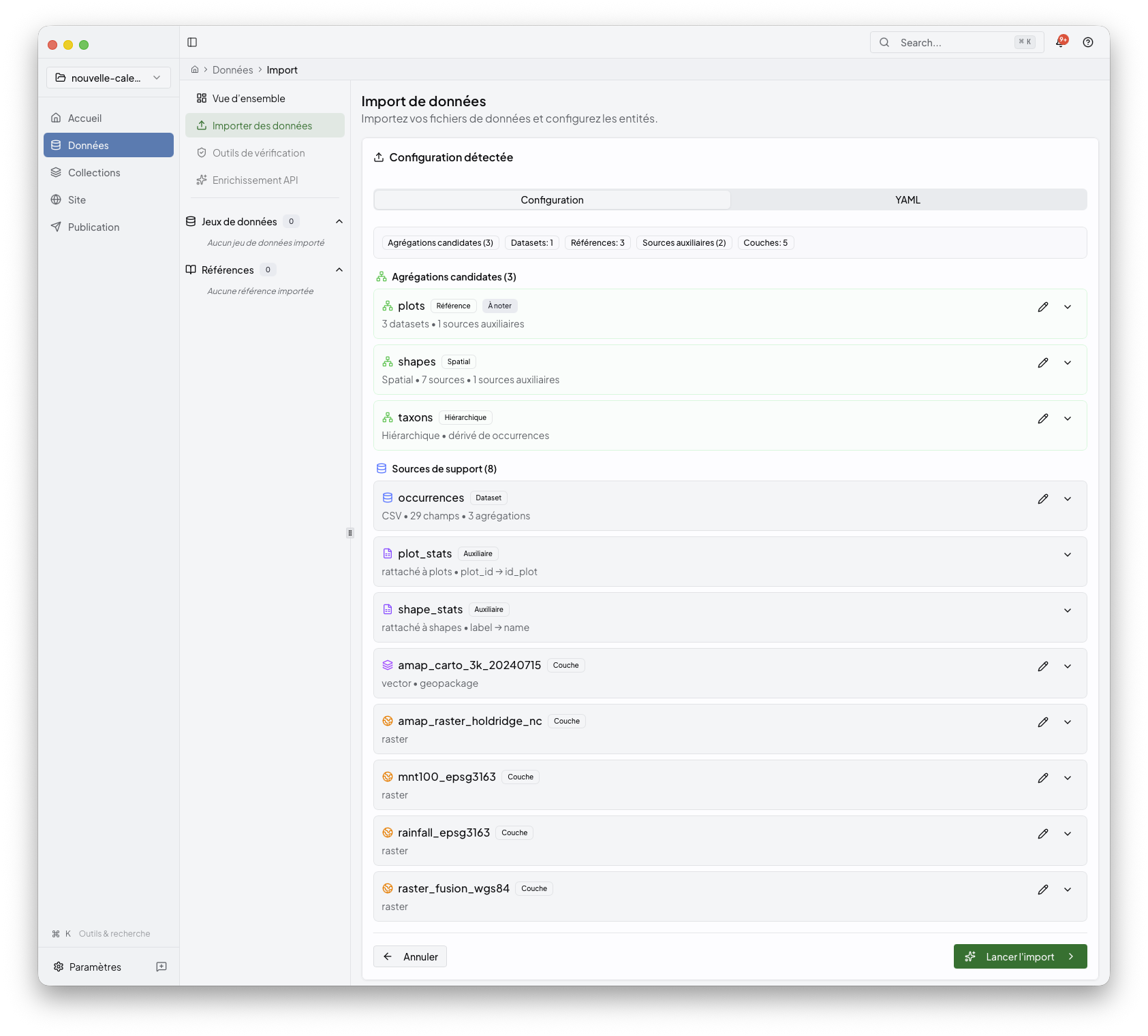
At this point you can:
confirm entity names
review identifiers and file roles
decide which sources become primary entities or supporting inputs
edit the generated YAML when you need more control
If the automatic detection has low confidence, the cockpit marks the item as needing review and explains the reason in the context panel. For example, it may ask you to confirm the file role, choose a stable identifier, or verify that two related files share the same identifier values.
The detailed configuration editor and YAML preview are still available from the advanced review panel, but they are no longer the first thing you need to read. Use them when you want to correct a detection or inspect the generated configuration.
Behind the UI, this stage is mostly shaping config/import.yml. The goal is
not to hand-edit YAML by default, but to understand that the review screen is
saving the same import structure the CLI can also use.
4. Run the import
Once the configuration looks right, start the import and follow the progress in the same workspace.
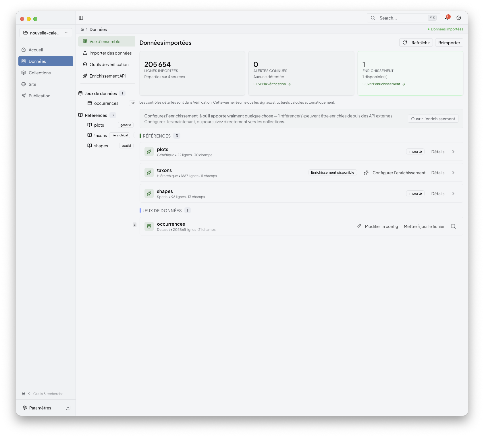
After a successful import, the project dashboard becomes the handoff point to the next stages:
inspect the imported entities
continue into collections.md
move later into site.md and publish.md
Optional follow-up: enrichment
Some imported references can expose enrichment as a later step. Keep that as a follow-up once the main import is stable; it is not required for the first pass through the desktop workflow.